Model Compression for Efficient Training & Inference of Large Language Models

Laith Zumot • 2025

Practical Model Compression

graph LR
    A[Model Compression] --> B[Pruning]
    A --> C[Distillation]
    A --> D[Quantization]
    A --> E[PEFT]

    B --> B1[Unstructured Pruning]
    B --> B2[Structured Pruning]
    B --> B3[Rank Reduction]

    C --> C1[Logit Distillation]
    C --> C2[Hidden-State Distillation]

    D --> D1[Post Training Quantization]
    D --> D2[Quantization Aware Training]

Quantization

  • Reduce precision of weights/activations to shrink memory & speed up math
    • e.g., BF16 → FP8.
    • Lower memory footprint → larger batch / context on same hardware
    • Higher arithmetic intensity → faster GEMMs / attention
    • Cheaper deployment on edge/CPU
  • PTQ (Post-Training Quantization)
    • No retraining; quick to try
    • Needs calibration data to estimate activation ranges
    • Schemes: per-tensor/per-channel, symmetric/asymmetric
    • Gotchas: outliers, distribution shift, layerwise sensitivity
  • QAT (Quantization-Aware Training)
    • Best accuracy under low bit-widths (fake-quant + STE)
    • Matches deploy time numerics (quant/dequant in-graph)
  • Common formats & typical use
    • FP8 (e4m3/e5m2): high throughput training/inference; mild loss
    • INT8: robust sweet spot for prod inference
    • MXFP4: used in GPT-OSS for MOE experts (MP).
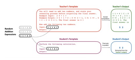
Quantization — calibration, scaling & pitfalls

  • Core knobs
    • Granularity: per-channel (kernels) > per-tensor
    • Ranges: min/max, percentile clipping, KL-based, EMA observers
    • Rounding: nearest vs stochastic; smooth quant for activations
  • Calibration goals
    • Estimate activation/weight ranges that minimize clipping & rounding error
    • Use representative samples (same domains/prompts/seq lengths as prod)
    • Track both quality (e.g., perplexity, accuracy) and latency/memory
  • Range estimation
    • Min–Max / AbsMax (fast; risk of outlier blow-up)
    • Percentile clipping (e.g., 99.9th) to tame long tails
    • KL-divergence / MSE minimization to pick bins
    • EMA observers during QAT for stable moving ranges
  • Scaling schemes
    • Symmetric (zero-point = 0): common for weights
      - scale = max(|x|) / qmax
    • Asymmetric (nonzero zero-point): common for activations
      - scale = (x_max − x_min) / (qmax − qmin)
    • Granularity: per-channel (weights) > per-tensor; group-wise for INT4
  • Outlier management
    • Keep sensitive parts in higher precision: embeddings, LM head, K/V proj
    • SmoothQuant-style activation smoothing (shift dynamic range into weights)
    • Weight-only quant (e.g., W8A16 / W4A16) to avoid activation quant error
  • Implementation tips
    • Static (ahead-of-time) quantization with calibration > dynamic on GPUs
    • Fuse ops (conv/linear + bias + activation) before quantization if possible
    • Align scales with kernel requirements (tile sizes, tensor cores)
    • For QAT: fake-quant + STE; freeze observers late; fine-tune LR ↓
  • Pitfalls & mitigations
    • Distribution shift between calibration & prod → recalibrate by traffic slice
    • Saturation in attention/LayerNorm paths → leave in FP16/FP32
    • Dequant overhead on small layers → quantize hot GEMMs first
    • INT4 regressions → use group-wise scales, try QAT/QLoRA, or back off to INT8
    • Sequence length sensitivity → calibrate at prod seq lengths
  • Validation checklist
    • A/B: task metrics (↓ perplexity Δ, ↑ exact-match) + latency/throughput + VRAM
    • Layerwise sensitivity sweep; opt-out layers that cause large drops
    • Save scales/observers with model artifacts; log calibration dataset hash

Distillation

  • Train a student model to match a teacher model’s output distribution (soft targets).

  • Loss (with temperature \(T\)): \[ \mathcal{L} = (1-\alpha)\,\mathrm{CE}(y, p_s) \;+\; \alpha\,T^2\,\mathrm{KL}\!\left(p_t^{(T)} \,\|\, p_s^{(T)}\right) \]

  • Backprop only through the student; the teacher is frozen.

  • Variants: use KL or JS divergence; mix in hard-label CE; schedule \(T\) or label smoothing.

  • Online distill: teacher forward + student forward/backward (higher GPU but no disk I/O).

  • Offline distill: cache teacher logits; cheaper GPU at train time but larger storage/I/O.

  • Issues:

    • Training cost: Expect ~20–30%+ extra memory for activations/gradients beyond raw parameter memory (depends on context length, batch size, kernels).
    • Exact logit matching can be restrictive; the student may imitate outputs without learning richer internals.
    • Students may not learn intermediate representations; consider feature/attention distillation or auxiliary losses.
    • length/verbosity bias from the teacher; mitigated with CE mixing, calibration, and data augmentation.
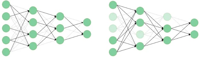
Post Training - Distilling 405B / 70B → 8B (Order-of-Magnitude)

  • Memory Footprints (FP16/BF16, params only)
Model Params Approx. Memory
Teacher (large) 405B ~810 GB
Student 8B ~16 GB
  • Activations & gradients: add ~20–30% overhead (implementation- and length-dependent).
  • Teacher inference-only memory (online distill):
    • 405B: ~1 TB+
  • Student training memory (8B, long context ~128k): ~160 GB
    • (model + activations/optimizer; depends on sharding/checkpointing).
  • Hardware Sketches
    • Teachers
      • 405B:
        • 16–24× H100 80GB, tensor/pipeline parallel
        • InfiniBand interconnect
        • ~2 TB system RAM
    • Student (8B)
      • 2× H100 with NVLink
      • ≥256 GB RAM host
      • Fits comfortably with mixed precision + gradient checkpointing

Pruning

  • Reduce params/FLOPs/VRAM; potential latency gains (esp. with sparse kernels).

  • How weights are pruned

    • Unstructured (element-wise): highest sparsity; requires efficient sparse kernels
    • Structured (channels/filters/heads): immediate speedups; lower flexibility
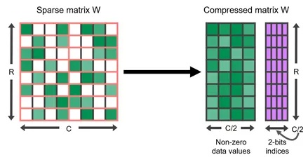
    • N:M sparsity (e.g., 2:4): HW-friendly pattern; good accuracy/speed trade-off
  • Which weights to prune

    • Magnitude-based (|w|, L1/L2): simple, strong baseline
    • Movement pruning (|Δw| during fine-tune): preserves changing weights
    • Gradient/Taylor saliency: |g·w| (first-order importance)
    • SNIP/GRASP (pre-train sensitivity analysis);
    • Optimal Brain Surgeon (2nd-order, costly)
    • Head importance via contribution/entropy; prune low-value heads
  • Scheduling

    • One-shot: prune once → (re)train (fast/risky)
    • Iterative/gradual: increase sparsity over steps
      • Example cubic schedule to target S*: S(t)=S*·(t/T)^3
# Pseudocode for gradual pruning
target_sparsity = 0.8  # 80% pruned
total_steps = 10000
for step in range(total_steps):
    current_sparsity = target_sparsity * (step / total_steps) ** 3
    prune_weights(model, current_sparsity)  # Remove smallest weights
    train_one_batch(model, data)

Pruning — Strategies

  • What counts as “prunable”?
    • Global Rank weights across all layers → prune globally. Maximizes sparsity.
    • Layerwise layer-specific thresholds to avoid over-pruning critical layers.
  • How to fix accuracy post-pruning
    • Retrain/Rewind: Fine-tune the pruned model; optionally revert to a pre-pruning checkpoint.
    • Optionally add distillation style loss (logits or hidden states) to mimic the original model’s outputs/logits during retraining
  • End-to-end workflow
    1. Establish baseline: task metrics, perplexity, latency/throughput, VRAM.
    2. Sensitivity sweep: per-layer sparsity curve (e.g., 0→90%) to find fragile blocks.
    3. Choose pattern: unstructured | structured (channels/heads) | N:M (e.g., 2:4).
    4. Set sparsity budget: global target + layerwise caps (protect embeddings/LN).
    5. Schedule: one-shot or gradual (e.g., cubic to S* over T steps).
    6. Prune & recover: brief fine-tune with small LR; consider distillation.
    7. Export & realize speed: use kernels that honor sparsity (structured / N:M).
    8. Validate in prod-like loads: seq length, batch size, mixed precision.
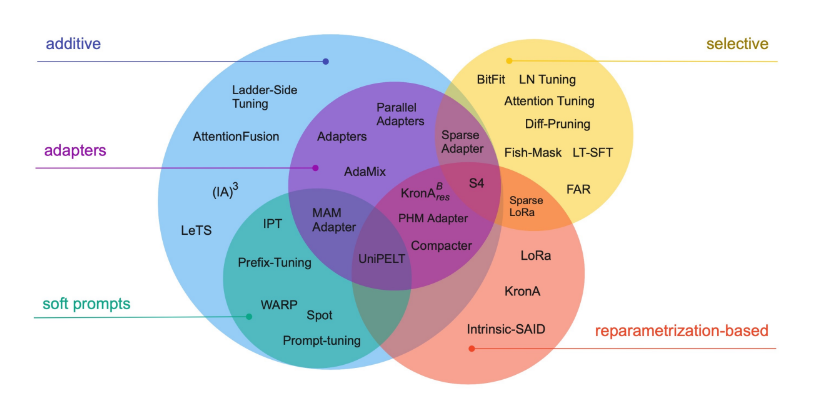
Pruning — Recovery

  • Recovery training
    • LR: 0.1–0.3× of fine-tune LR; no warmup or very short.
    • Masking:
      • Fixed-mask (recommended): Keep pruned weights at 0 permanently → deterministic deployment.
      • Re-growth (Rigged Lottery): Allow new connections early, then freeze later.
        • RigL dynamically re-grows pruned connections and prunes less important ones cyclically
        • Inspired by the Lottery Ticket Hypothesis: It searches for high-performing sparse subnetworks by “rigging” the connectivity in favor of high-potential weights.
    • Regularizers:
      • L1-loss (unstructured): Encourages more zeros.
      • Group Lasso (structured): Penalizes entire channels/groups
    • Distillation (optional):
      • add KL(logits) and/or feature loss to preserve behavior.
    • Checkpoints:
      • Rewind/Reset weights to a pre-prune checkpoint mid-recovery if unstable.
# Pseudocode for RigL_training
def RigL_training(model, sparsity_ratio, update_freq, total_steps):
    initialize_sparse_mask(model, sparsity_ratio)  # Random or pruned
    for step in 1...total_steps:
        train_one_batch(model)  # Optimize active weights
        
        if step % update_freq == 0 and step < 0.8 * total_steps:
            prune_mask = bottom_k_weights(model, prune_ratio) # Smallest weights
            regrow_mask = top_k_gradients(model, prune_ratio) # Pruned weights w/highest |∇L|
            update_mask(model, prune_mask, regrow_mask) # Swap connections

Pruning — Caveats

  • Structured pruning specifics
    • Dimensions Matter:
      • Prefer removing entire heads/MLP channels to get immediate kernel wins.
      • Example: Removing only 2 attention heads reduces num_heads and subsequent projection sizes.
    • Post-Surgery Calibration:
      • Run 10–100 inference steps to recompute network statistics (e.g., LayerNorm means).
    • Hardware Gains:
      • Removing entire blocks unlocks native kernel optimizations (e.g., cuDNN group conv).
  • Caveats & gotchas
    • Sparsity ≠ speed
      • Unstructured sparsity benefits only with sparse accelerators (e.g., Ampere GPUs)
      • Structured/N:M always wins for latency.
    • Over-tokenized (Llama3) may have limited pruning headroom.
    • Excessive attention-head pruning can harm long-context/generalization.
    • Prune-then-quantize usually more stable than quantize-then-prune; if mixing, plan QAT.
    • Do NOT prune embeddings/LayerNorm/residual dims
    • For deploy speedups, match your HW: structured or N:M > random sparsity
    • Typical safe starts: 30–50% structured OR 60–90% unstructured

PEFT

  • Parameter-Efficient Fine-Tuning = freeze the base model and train a small set of extra parameters (adapters, low-rank deltas, prompts).
    • Tiny trainable footprint (often <1% of params) → fits on modest GPUs
    • Faster training & lower memory/IO; checkpoints are small & swappable
    • Multi-task: keep multiple adapter heads for different domains
  • Core patterns
    • Adapters: small bottleneck MLPs inserted in blocks
    • LoRA/DoRA: learn low-rank (or decomposed) deltas on weight matrices
    • Prefix/Prompt/Soft-prompt: learnable tokens prepended to inputs/keys
    • IA³ / BitFit: learn per-feature scalars (attn/FFN) or just biases

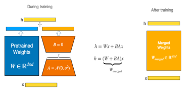
LoRA Deep Dive — mechanics

  • Freeze base model weights:
    \[\begin{aligned} $W \in \mathbb{R}^{d_\text{out} \times d_\text{in}}$ \end{aligned}\]

  • Learn low-rank weight delta:
    \[\begin{aligned} W' &= W + \Delta W \\ \Delta W &= BA \\ \end{aligned}\] \[\begin{aligned} where: $A \in \mathbb{R}^{r \times d_\text{in}}$ , $B \in \mathbb{R}^{d_\text{out} \times r}$, $r \ll \min(d_\text{in}, d_\text{out})$ \end{aligned}\]

  • Apply adaptive scaling:
    Forward pass uses: \[Wx + \frac{\alpha}{r} B(Ax)\] (\(\alpha\) = tunable scaling constant)

  • Optional regularization:
    LoRA Dropout applied directly to input \(x\)

LoRA Deep Dive — sample code

# Pseudocode for LoRA
class LoRAparam(nn.Module):
    def __init__(self, features_in, features_out, rank=1, alpha=1, device='cpu'):
        super().__init__()
        self.lora_A = nn.Parameter(torch.zeros((rank,features_out)).to(device))
        self.lora_B = nn.Parameter(torch.zeros((features_in, rank)).to(device))
        nn.init.normal_(self.lora_A, mean=0, std=1)
        self.scale = alpha / rank
        self.enabled = True

    def forward(self, original_weights):
        if self.enabled:
            # Return W + (B*A)*scale
            return original_weights + torch.matmul(self.lora_B, self.lora_A).view(original_weights.shape) * self.scale
        else:
            return original_weights

def linear_layer_parameterization(layer, device, rank=1, lora_alpha=1):
    features_in, features_out = layer.weight.shape
    return LoRAparam(features_in, features_out, rank=rank, alpha=lora_alpha, device=device)
 
nn.utils.parametrize.register_parametrization(net.linear1, "weight", linear_layer_parameterization(net.linear1, device))

LoRA Deep Dive — configs

  • Where to apply (LLMs)
    • Attention: q_proj, k_proj, v_proj, o_proj
    • MLP: up_proj / down_proj / gate_proj
  • Key knobs
    • rank r: 4–64 typical; higher r = more capacity/memory.
    • lora_alpha: 8–64; acts like gain. Pair with r (e.g., r=16, α=32).
    • lora_dropout: 0.0–0.1; helps regularize on small data.
    • bias: usually “none”; keep base biases frozen.
  • Training config (rules of thumb)
    • Optimizer: AdamW (β=(0.9,0.999)), wd=0.0–0.1 (often 0 for LoRA).
    • LR: 1e-4 to 5e-4 (instruction tuning) or 5e-5 to 2e-4 (task/classif).
    • Warmup 3–5%; cosine or linear decay; grad clip 0.5–1.0.
    • Mixed precision (BF16/FP16), gradient checkpointing for long seqs.
    • Small KD logits loss can stabilize instruction-following.
  • QLoRA (LoRA on 4-bit bases)
    • Weight quantization: load base in 4-bit NF4 (normal float 4) with double quantization; compute in BF16/FP16.
    • Train LoRA adapters in FP16/BF16; base remains frozen INT4 → huge VRAM savings.
    • Use paged optimizers (e.g., paged AdamW) to avoid OOM with long contexts.
    • Keep embeddings & output head at higher precision if quality dips.
    • Typical config: r=16–64, α=32–64, dropout=0–0.05; target q,v,(o,up/down) first.
  • Deployment
    • Inference can merge (W) into (W) (for dense FP weights) or keep adapters separate (preferred with quantized bases).
    • Export only adapter checkpoints for lightweight shipping.

Other PEFT Variants — Adapters, Prefix/Prompt, IA³, BitFit, DoRA

  • Prefix / Prompt / P-Tuning v2
    • Prompt-Tuning: Learns soft prompts (trainable embeddings) exclusively at the input layer.
      • weaker performance on large domain shifts (Prompt-Tuning)
    • Prefix-Tuning: Learns task-specific K/V vectors across multiple layers, offering higher capacity than Prompt-Tuning. -increased sequence length costs (Prefix-Tuning).
    • Recipe: 20–100 virtual tokens; Prefix on deeper tasks, Prompt for light retargeting.
  • IA³ (Intrinsic SA Scalings)
    • Learns feature-wise scaling vectors applied multiplicatively to weights in attention (Q,K,V) and FFN layers.
    • Minimal parameters (<1% of base model) and near-zero latency overhead
    • Recipe: enable scalars in attn proj & FFN gating; LR≈1–2e-4; wd=0.
  • BitFit
    • Train only biases.
    • Pros: microscopic checkpoints; surprisingly strong when task ≈ pretrain.
    • Cons: limited capacity on hard domain shifts.
    • Recipe: unfreeze biases + LM head; LR≈1–3e-4; early stop.
  • Adapters (Houlsby / Pfeiffer)
    • Insert small bottleneck MLPs in blocks; train only adapter params.
      • Houlsby, two adapters sequentially within one layer of the transformer, one after the multi-head attention and one after the FFN sub-layer, while
      • Pfeiffer et al., adapter is inserted only after the FFN “add & layer norm” sub-layer.
    • Recipe: insert after attention & MLP; b=32 start; LR≈1e-4; wd=0; warmup 3%. GELU activation, and near-identity initialization
  • DoRA (Decomposed LoRA)
    • Decompose weight into magnitude × direction; learn low-rank updates to direction.
    • Often more stable than vanilla LoRA, esp. with quantized bases.
    • Recipe: replace LoRA with DoRA on sensitive mats (q,v); r=8–32, α=16–32.
  • Choosing among them (quick cues)
    • Tiny budget / many tasks → Prompt/Prefix, BitFit, IA³
    • Need stability & modularity → Adapters
    • Max perf/param → LoRA/DoRA (add QLoRA if VRAM-bound)

Example of LoRA FT

A example LoRA FT to add Mojo language to deepseek coder

Citations & Further Reading

Citations & Further Reading

Images created w Gemeni

“Model Compression and Efficient Inference for Large Language Models: A Survey” https://arxiv.org/html/2402.09748v1
“Efficient Compressing and Tuning Methods for Large Language Models: A Systematic Literature Review” https://dl.acm.org/doi/10.1145/3728636
“Advances and Challenges in Large Model Compression” https://dl.acm.org/doi/fullHtml/10.1145/3675417.3675487

[Q1] ZeroQuant: Yao et al. 2022 https://arxiv.org/abs/2206.01861
[Q2] Outlier-Suppression: Wei et al. 2022 https://arxiv.org/abs/2209.13325
[Q3] Bondarenko et al. 2023 “Quantizable Transformers” https://arxiv.org/abs/2306.12929
[Q4] BinaryBERT: Bai et al. 2021 https://arxiv.org/abs/2109.12934

[D1] Step-by-Step Distillation: Hsieh et al. 2023 https://aclanthology.org/2023.findings-acl.432
[D2] GKD: Agarwal et al. 2023 https://arxiv.org/abs/2306.13649
[D3] LLM-KD: Gu et al. 2023 https://arxiv.org/abs/2306.08543

[P1] LLM-Pruner: Ma et al. 2023 https://arxiv.org/abs/2305.11627
[P2] Optimal BERT Surgeon: Kurtic et al. 2022 https://arxiv.org/abs/2203.07259
[P3] What Matters in Structured Pruning: Santacroce et al. 2023 https://arxiv.org/abs/2302.03773
[P4] RigL: Evci et al. 2020 https://arxiv.org/abs/2005.07233

[L1] LoRA: Hu et al. 2022 https://arxiv.org/abs/2106.09685
[L2] QLoRA: Dettmers et al. 2023 https://arxiv.org/abs/2305.14314
[L3] Adapters: Houlsby et al. 2019 https://proceedings.mlr.press/v97/houlsby19a.html

Thank You for Reading!